
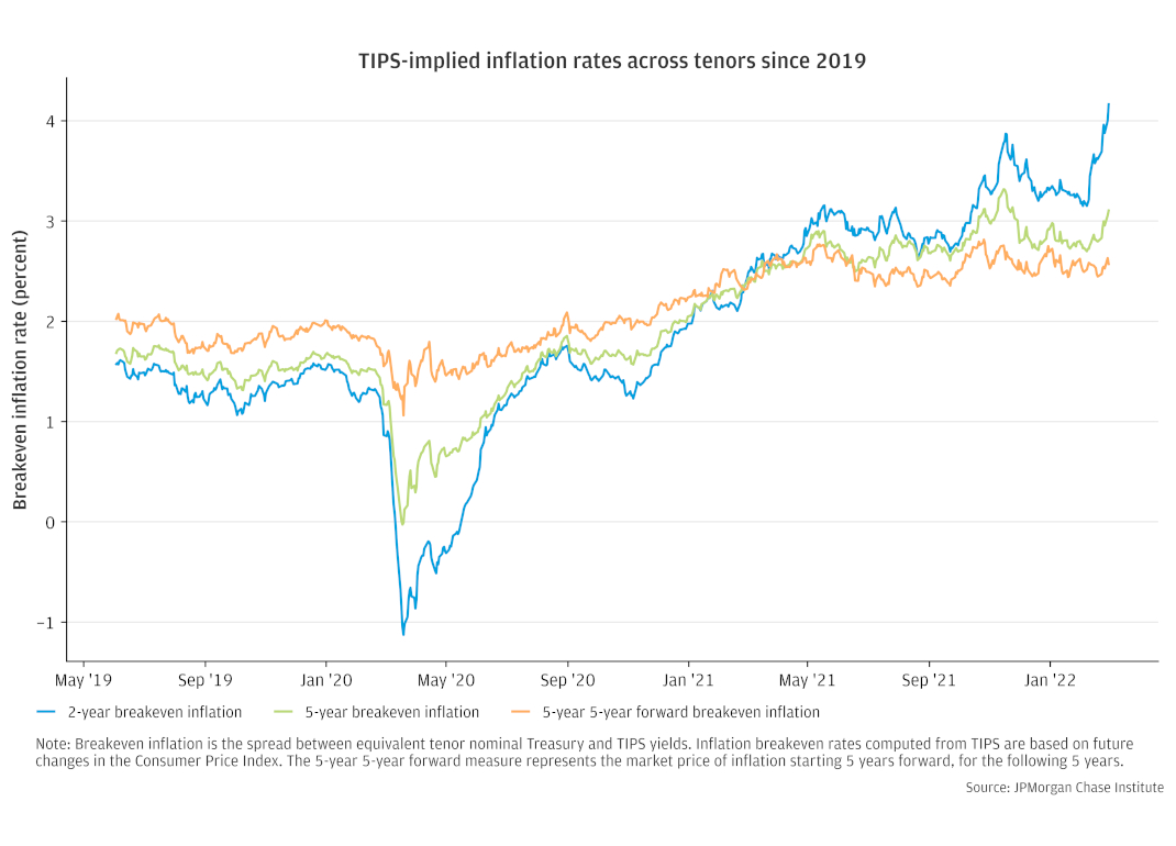
Figure 1: Market-based expected inflation measures have risen notably in the short-term, while longer-dated measures remain largely stable.

Creating thriving communities together
See how our clients and partners—from small business owners to workforce training leaders—work with JPMorganChase to drive meaningful impact and economic growth where they live and work.
Learn moreLatest news

Veteran’s Unconventional Path to Landing her Dream Job in Tech
U.S. Army Veteran Ashley Wigfall transitioned to a civilian role and charted her path to technologist through mentorship and skills training at the JPMorgan Chase tech hub in Plano, Texas.
Learn more
Findings
Since the onset of the COVID-19 pandemic, the U.S. economy has experienced inflation fluctuations that haven’t been seen for decades.1 Volatility in the price levels of goods and services may contribute to persistent changes in households and businesses’ inflation expectations, a limiting factor for policymakers seeking to strengthen the economic recovery. Surveys and financial markets provide evidence of evolving expectations. However, both sources of information are imperfect, leaving policymakers with noisy signals to guide policy. Market-based indicators—such as those based on U.S. Treasury Inflation Protected Securities (TIPS)—have the advantages of being priced by investors with “skin in the game” and are updated in real-time. In this insight, we use granular transaction data in the TIPS market to characterize sources of noise policymakers can consider when assessing inflation expectations.
Since the current economic recovery began in mid-2020, the market has sent a strong signal of higher inflation expectations. The rise has been most pronounced in measures covering short time horizons, e.g. over the next 2 years, while longer-dated measures have remained comparatively well-anchored (see Figure 1). These dynamics are consistent with the view that monetary policy would respond sufficiently to prevent a sustained overshoot of inflation above the Federal Reserve’s 2 percent objective, affirmed by the pivot in policymaker communications since late 2021.2
Figure 1: Market-based expected inflation measures have risen notably in the short-term, while longer-dated measures remain largely stable.
We find that institutional investor trading can drive measures of inflation expectations based on TIPS—potentially distorting their signal for expectations—but the impact from observed trading is usually small. Our estimates indicate that the price impact of TIPS trading flows is higher when overall market volatility is elevated. Conversely, flows have an imperceptible effect, on balance, when volatility is below average. The rise in market-implied inflation from mid-2020 through late 2021 may have been amplified by trend-chasing activity, although the price impact of trading in our data explains, at most, one-fifth of the increase. Pockets of investors tend to trade systematically either with, or against, price movements, suggesting conditions facing these participants can lead to market movements that exaggerate or underestimate true changes in expectations, respectively. Our analysis supports the view that the TIPS market is highly informative of inflation expectations, but policymakers should consider distortions resulting from trading behavior when interpreting market signals, especially when volatility is elevated.
We organize our analysis around four findings.
Finding 1. Institutional investor trading activity affects indicators of inflation expectations, but distortions are usually modest when volatility is contained.
Finding 2: Trend-chasing flows contributed modestly to the rise in inflation pricing since mid-2020.
Finding 3. Investor flows help explain the sharp divergence in relative TIPS pricing during March 2020, in which less-liquid securities deeply underperformed amid extreme market volatility.
Finding 4. Market participants that usually trade against prevailing price action initially bought TIPS as their prices fell in March 2020, however, their purchases were small and began to reverse by the peak of the crisis.
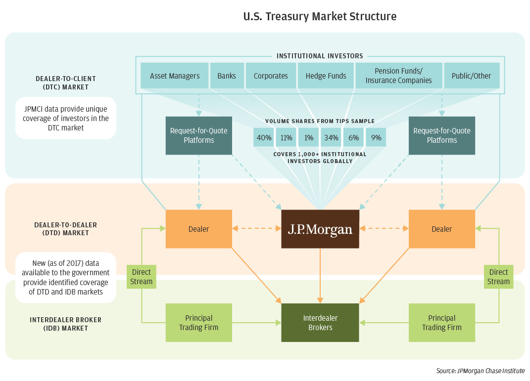
Our unique lens comes from de-identified data about institutional investor trading in financial markets. The data used in this analysis cover over 1000 global institutional investors’ transactions in TIPS with the Markets Division of J.P. Morgan’s Corporate and Investment Bank from 2013 through late 2021. Trades worth about $1 trillion in gross volume form the core sample.
Our data provide a unique look into the dealer-to-client market for TIPS,3 complementing a dataset of Treasury market transactions available to government officials since 2017, Trade Reporting and Compliance Engine (TRACE) for Treasuries. The infographic below shows the perspective of our data in the context of the overall Treasury market structure.4 An important feature of our data—a panel data perspective with investor attributes—is a crucial element differentiating our analysis from the U.S. government’s dataset, which lacks detailed information of the end-investors trading in the dealer-to-client market. Our ability to follow individual investor’s activity over time aids our categorization of trading activity, supporting price impact estimates (introduced in Finding 1) and aggregated systematic flow calculations (described in Finding 4).
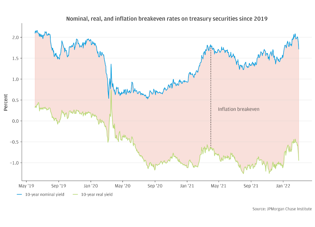
The main indicator of future U.S. inflation priced in bond markets is the difference between interest rates on standard (nominal) Treasury securities and those indexed to inflation: Treasury Inflation Protected Securities (TIPS).5 The return on TIPS is a combination of a “real” yield, representing the gain in purchasing power over a period of time, plus a rate tied to increases in the Consumer Price Index (CPI). The gap between the market yield on nominal Treasuries and the real yield of TIPS of the same maturity date is the rate of CPI-based inflation above which an investor would be better off to own TIPS. For this reason, it is termed the “breakeven” rate of inflation, depicted in Figure 2.
Figure 2. The difference between the yields on standard ‘nominal’ Treasury securities and TIPS represents the outlook for inflation.
Under simple financial theories with no transactions costs, the Treasury market would perfectly reflect the inflation rate expected by investors. In practice, however, distortions of market prices from expectations can come from numerous sources. For example, TIPS are less liquid than their nominal counterparts, suggesting the relevance of a liquidity discount which can vary over time. Meanwhile, the value of protection against high (or low) inflation outcomes can influence breakeven rates through risk premia that depend on the perceptions of traders.6 Reliably parsing market prices to differentiate expectations from risk premia is challenging and leaves policymakers with imprecise knowledge of true inflation expectations. We bring new granular data to the topic.
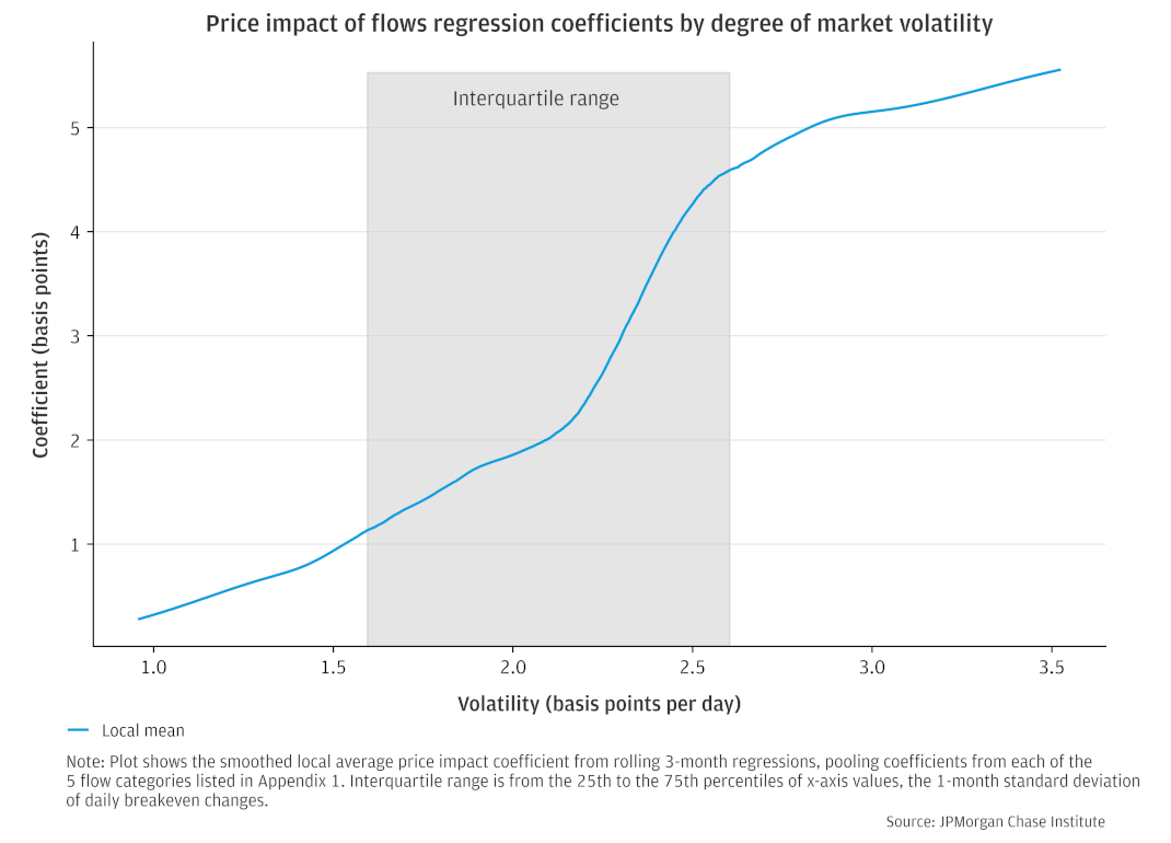
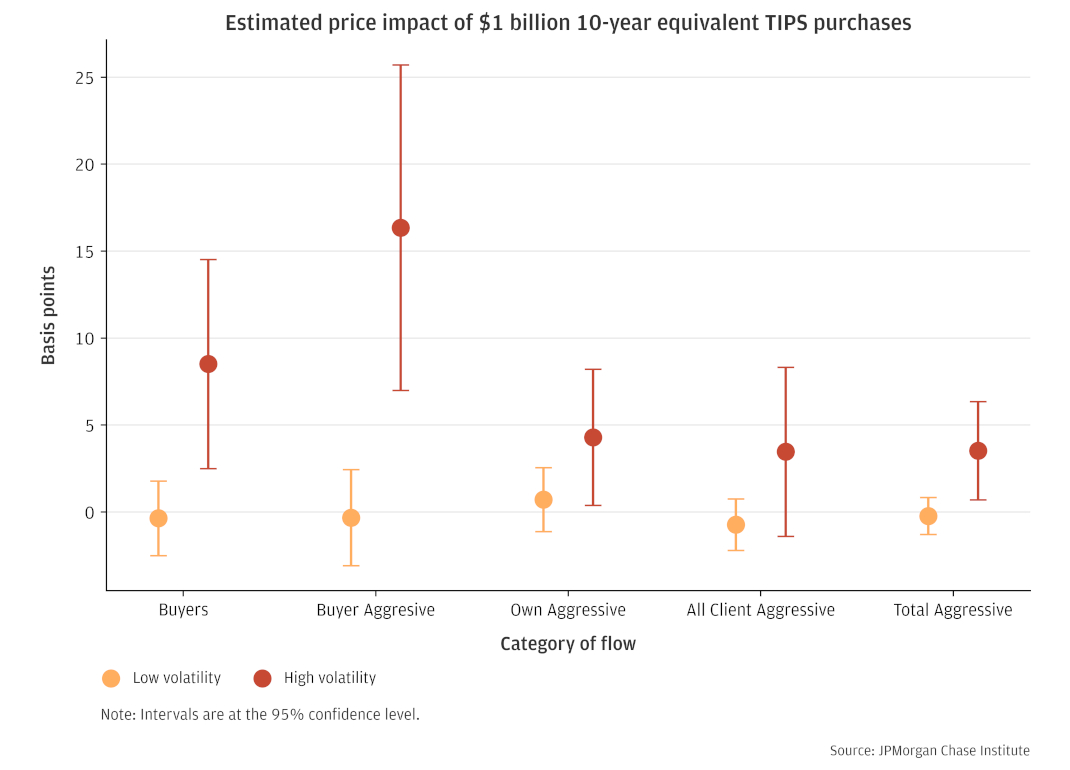
We find a correlation between trading activity and changes in inflation breakeven rates that helps explain fluctuations after controlling for changes in other market prices. Investor purchases in our data of $1 billion in TIPS—measured in 10-year equivalents—are associated with increases in inflation breakevens from just above 0 to 5.5 basis points, depending on the degree of market volatility (see Figure 3).7 The below box: Estimating price impact from flows data details our methodology.
Traditional views of time-varying liquidity are consistent with the positive relationship we find between market volatility and price impact of flows.8 The magnitude of the coefficients, however, are more difficult to compare with prior research on Treasuries, given differences in the data, time periods, methodology, and underlying markets across studies. Estimates of price impact in nominal Treasuries used to estimate the effects of Fed asset purchases—when scaled to the size of the TIPS market—suggests price impact of about half of one basis point per $1 billion in ten-year TIPS equivalents.9 Since a given flow in our data may reflect a larger transfer of risk that could be spread across multiple market makers, our central estimate of 1 to 2 basis points per $1 billion (when volatility is close to its average level) is not directly comparable to this figure. Our price sensitivity estimates would be roughly in line with the literature on Large Scale Asset Purchases (LSAP) under the assumption that flows in our data represent, on balance, a subset of risk transfers that are spread across a few or several dealers.
Figure 3. The impact of flows on market-based inflation expectations is greatest in volatile markets.
Relative to typical volatility in the market, our identification method attributes a limited amount of price movement to flows. From 2013 to 2019, the average one-day change in the 10-year inflation breakeven rate was about 2 basis points. By comparison, a one standard deviation increase in TIPS purchases would shift the breakeven rate upward by less than a quarter of a basis point in the direction of the aggressor trading.10 We view this evidence as largely consistent with the view that finds the TIPS market highly informative of changes in expectations, but we recognize the need to consider market distortions.11
Since every trade involves a buyer and a seller, analysis of the direction of the trading activity, or flow, requires identification of the initiator, or “aggressor,” of the trade. On the other side of the transaction is the trader providing either the security or cash demanded, which we refer to as the “provider.” Since longer-term TIPS carry more interest rate risk than TIPS with shorter time-to-maturity, we normalize trading volumes by the amount of risk transferred (e.g., net dollar value of a basis point, sometimes termed net DV01) and convert volumes to 10-year equivalents.
After parsing our data to identify aggressor trades—as described below—we run Ordinary Least Squares (OLS) regressions of the following form to estimate of βf, an indicator of the price impact of flows. In our baseline specification, we control for changes in nominal yields (n) in basis points, crude oil prices (c) in percent, and the Cboe Volatility Index also known as the VIX (v) in index points.
ΔBEt = βn Δnt + βc Δct + βv Δvt + βf ft + et
We measure time-varying price impact by conducting sub-sample analysis (depicted in Figure 1) and use interaction terms between flows and volatility, as reported in Appendix 1.
Aggressor flow identification
We use multiple approaches to infer the aggressor side of a trade. The task is challenging, because most TIPS transactions do not occur on exchange-like venues, where the trade price relative to the bid and ask prices helps identification. Our methods contend with this difficulty by using additional data about the context of the trade to identify which counterparty was most likely the aggressor.
We use the methodology developed in Finding 1 to estimate how much trading activity may have influenced the rise in breakevens from mid-2020 to late 2021. We find that aggressor flows from certain investors contributed notably to the rebound in breakevens, explaining about 30 basis points of the 160 basis point rise from June 2020 through October 2021, as illustrated in Figure 4. The category of trades we term “Aggressive Buyer” flows14 (the box above, Estimating price impact from flows data, defines the groupings) drive the highest predicted flow impact. The estimate applies the 2013-19 price impact coefficient to flows observed since mid-2019.
Figure 4. Over the COVID period, flows categorized as ‘Aggressive buyer’ add predictive power to a model of breakeven inflation.
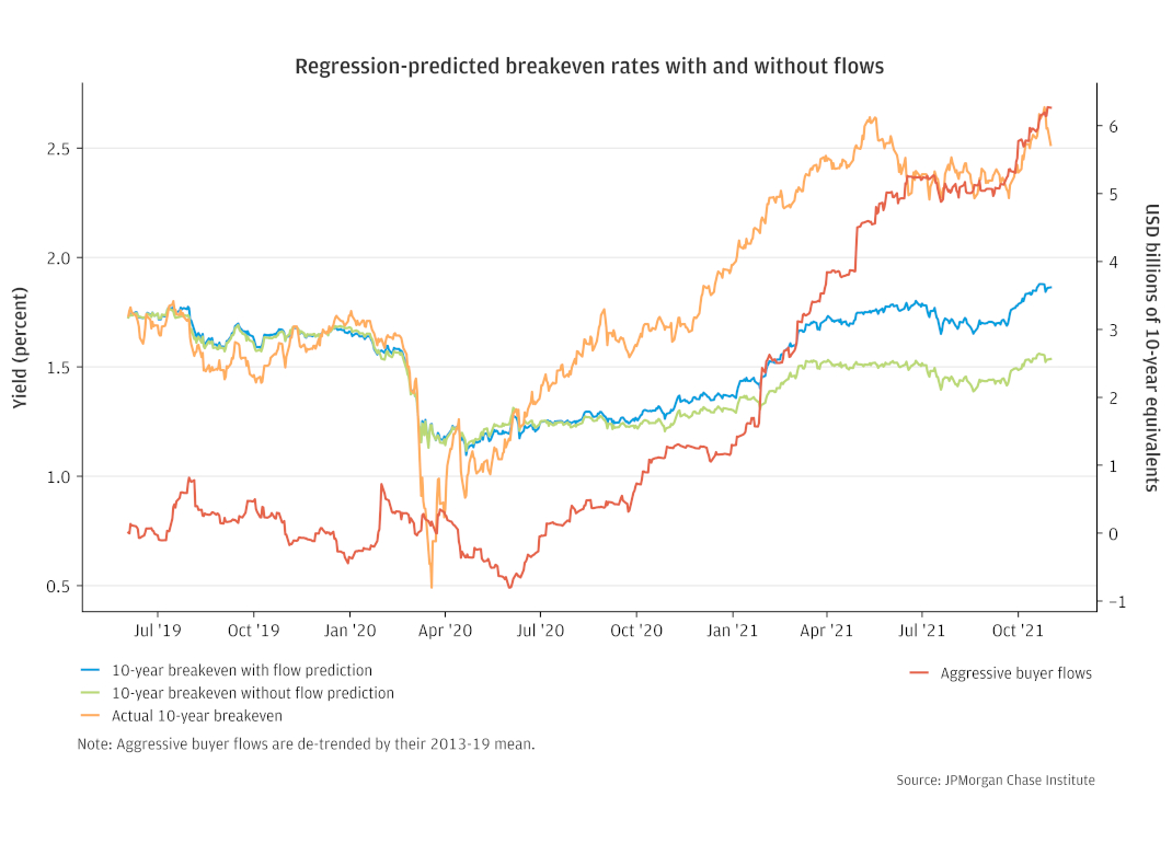
Interpreting dynamics over this period, however, is challenging for at least two reasons. First, the Fed’s large scale asset purchases likely altered the behavior of large dealers—particularly, primary dealers from which the Fed buys Treasuries—and their client counterparties. Indeed, in order to source securities to sell to the Fed, dealers need to make purchases in the market, which can tilt the net flows of clients towards selling. Second, higher volatility and uncertainty regarding inflation may have made dynamics observed over the in-sample period less applicable out-of-sample.
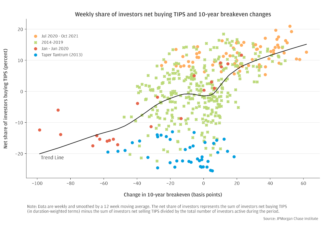
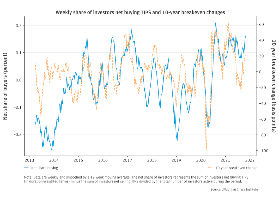
The trading behavior observed since the onset of COVID in early 2020 is consistent with prior episodes featuring large moves in Treasury yields. Investors in TIPS exhibit a trend-chasing pattern consistent with “herding.” As depicted in Figure 5, the share of institutional investors buying TIPS—in counts, not dollar values—increased alongside rising inflation breakeven rates and vice versa. The correlation between the two variables was 0.51 over the 2013-21 period.
The net number of investors buying TIPS dipped during the peak of the COVID crisis as breakeven rates collapsed. From mid-2020 through late-2021, the turnaround aligned with a prevailing imbalance of buyers outnumbering sellers. A previous episode of sharp outflows from the TIPS market—the 2013 Taper Tantrum, in which the 10-year breakeven rates fell approximately 70 basis points in 3 months—featured a similar dynamic; however, selling observed during that period was even stronger and more sustained than usual. A potential explanation for that period is the sharp shift from open-ended Fed asset purchases, after years of monetary stimulus.
Figure 5a and 5b. Trend-chasing activity—measured by the numbers of traders moving in the same direction—has been a pervasive dynamic in the TIPS market since COVID and in prior episodes.
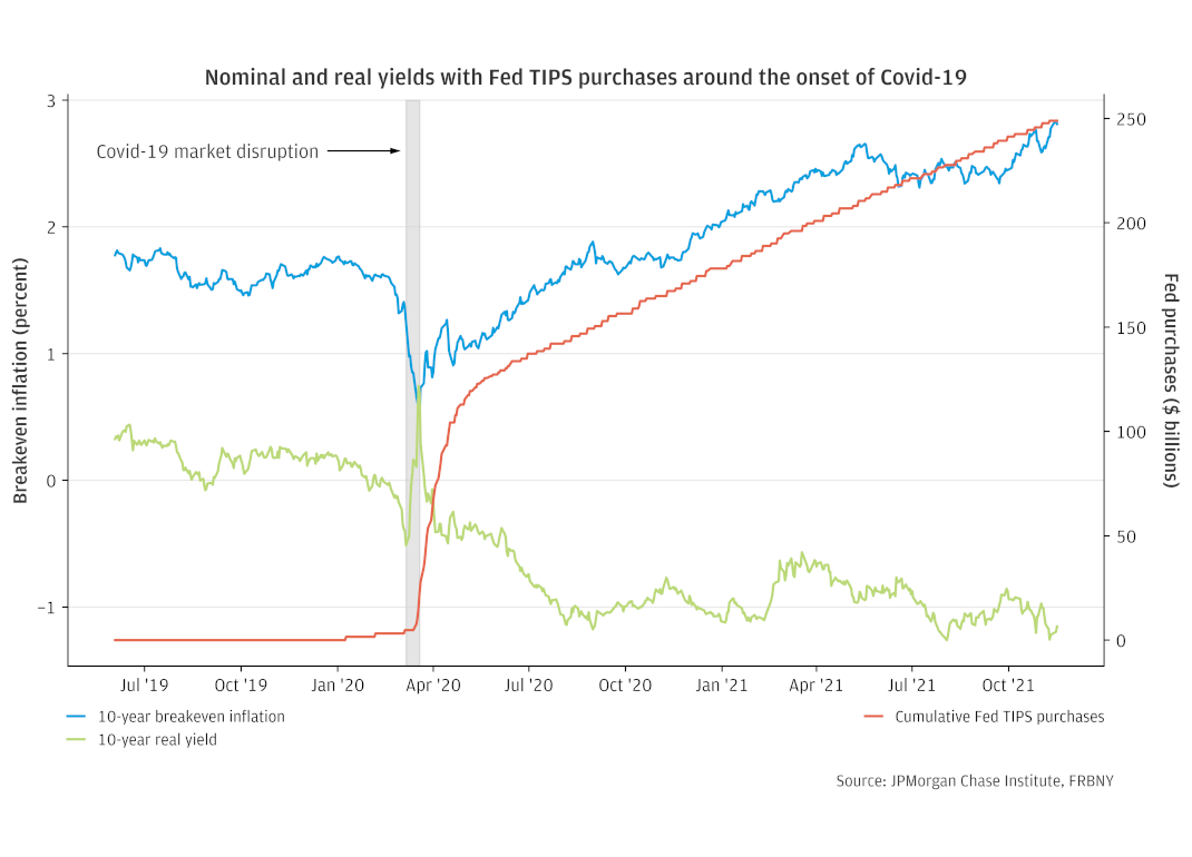
The rise in volatility across markets due to the COVID pandemic started in February 2020 and exploded in March. Treasury yields had been falling alongside declines in the stock market for two weeks until March 9, as the implications of spreading infections and the near-term economic fallout became clear. However, from March 9 to 18, most Treasury yields began rising and the deterioration in market liquidity accelerated, prompting aggressive Fed asset purchases to restore market function (see Figure 6). Given the focus of this analysis on inflation, we focus on TIPS. An interagency group of official sector policymakers and researchers provide an account of the episode centered on nominal Treasuries, enshrined in IAWG (2021).
Figure 6. The sharp March 2020 volatility in the broader Treasury market prompted large asset purchases by the Federal Reserve that included TIPS.
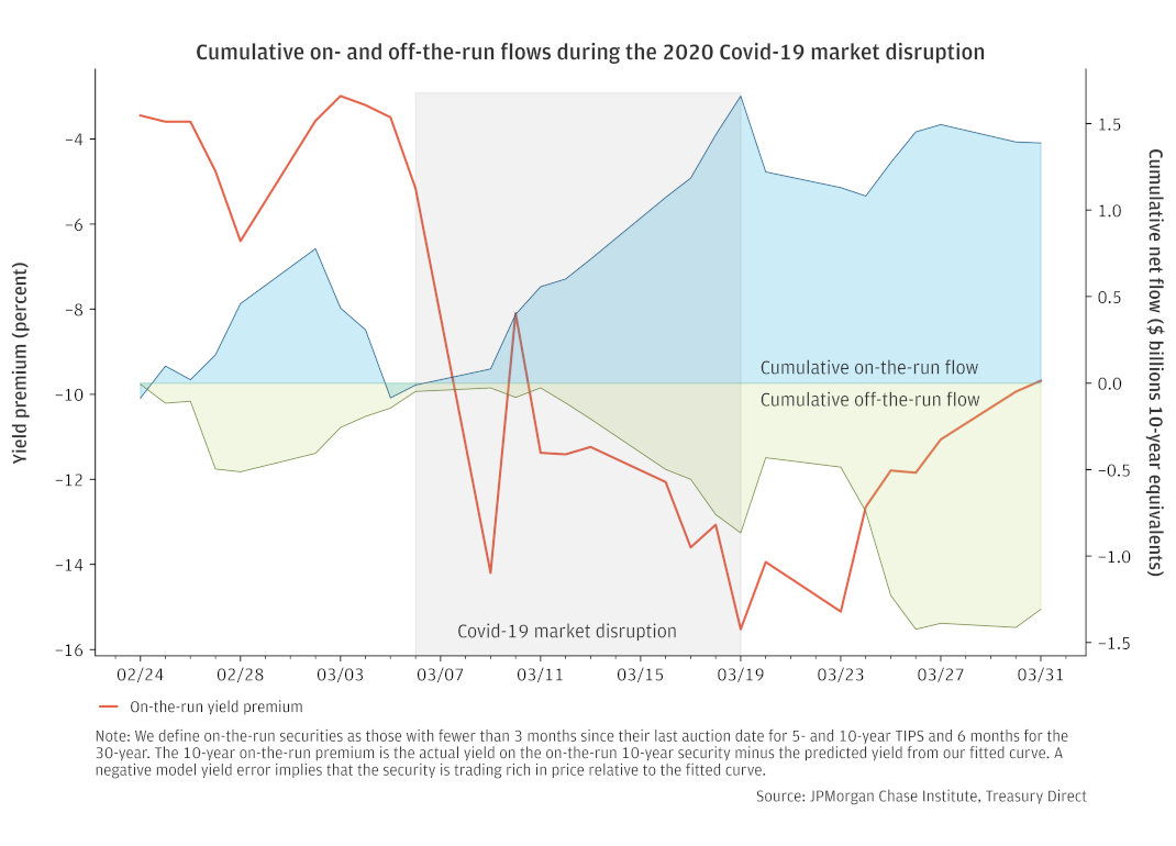
The extreme volatility in the overall yield curve was accompanied by stark divergences between the prices of different TIPS instruments that typically trade in nearly lockstep, due to their closely related cash flows. Investors have the choice to hold more recently issued Treasury securities—referred to as “on-the run”, or less recently issued securities, referred to as “off-the-run”. Gaps between these two sets of securities widened sharply as market volatility spiked, a sign of sharply deteriorating liquidity.
Our data help explain these trends. Investor sales of off-the-run TIPS coincided with purchases in more liquid on-the-run securities, depicted in Figure 7. During the two-week period of peak volatility, almost every trading day featured sales of off-the-runs and purchases of on-the-runs among institutional investors vis-à-vis J.P. Morgan. While some market participants took advantage of the opportunity to buy TIPS at depressed prices, they did so in the most liquid securities, leaving other investors to sell less liquid securities at relatively distressed values.
Figure 7. During the days of peak market volatility around the beginning of COVID, investors generally purchased more liquid on-the-run TIPS, while selling less liquid off-the-run TIPS.
A substantial portion of market participants in our sample trade in a systematic way, either buying TIPS as breakeven inflation rises or vice versa consistently over time. Market participants that trade in a correlated way with prices—either a positive or negative correlation—represent over half of TIPS market participants that trade actively in our sample and 80 percent of active market participants’ flows.15 To categorize investors, we run client-level regressions of flows against TIPS performance, measured by breakeven rates (capturing TIPS performance relative to nominal Treasuries) and by real yields (capturing raw TIPS price changes). Appendix 2 details the categorization methodology.
Investors that trade in the prevailing market direction we term “trend-chasers.” This category of investors augments the analysis in Finding 2, in which we document herding behavior in the direction of price movements, a pattern that emerges when averaging trading patterns across market participants. The categorization method discussed in this Finding makes the additional requirement of repeated behavior at the market participant level. We label investors who frequently trade in the opposite direction of prices “contrarians.” These two sets of investors inherently exert counterbalancing forces on the market, with the former tending to exacerbate price movements and the latter dampening volatility.
As documented by an extensive IAWG report, a key contributor to Treasury market volatility in March 2020 was investor selling in a “dash for cash.”16 Flows from the contrarian category should typically counteract such a force. Figure 8 depicts contrarian investor behavior in TIPS during the episode. Indeed, contrarians initially traded against the sharp declines in inflation breakevens, buying TIPS as expected. However, days before large Fed purchases began, contrarians diverged from predicted behavior and started to sell when prices were at their lowest point.
Figure 8: Contrarian TIPS investors, who typically trade against price changes, acted as expected until mid-March 2020 when they unwound earlier purchases in the face of extending market deterioration.
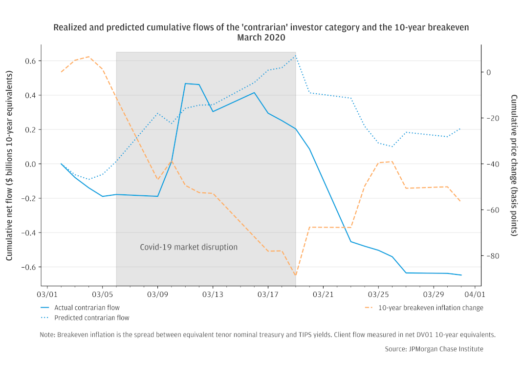
We interpret the pattern of flows during March 2020 as suggestive of limitations to contrarian trading as a market stabilizer. Even if contrarian investors are willing take on risk by buying assets as prices decline, extended price movements could lead to losses on those positions. This could possibly trigger position unwinds, degrading the ability for contrarians to act as a volatility buffer in extreme circumstances.
Following Fed intervention, contrarian investors resumed their prior trading behavior, selling into the rebound in inflation breakeven rates between March and September 2020 (see Figure 9). The general pattern continued through most of 2021. In effect, contrarian selling provided the counterpoint to Fed purchases, and as documented in Finding 2, aggressive purchases by trend-chasing investors.
Figure 9: Trading by contrarian investors in TIPS provided supply in the wake of aggressive Fed asset purchases in 2020, but have since been fairly balanced against trend-chasers.
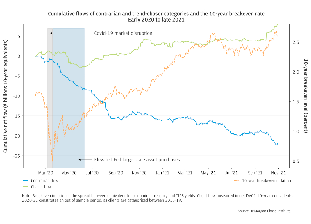
Looking forward, imbalances between systematic trading categories have the potential to cloud the market’s signal for inflation expectations. To the extent trend-chasing dominates contrarian flows, price movements may overshoot true changes in expectations. On the other hand, contrarians tend to keep markets range-bound, potentially leading the market to understate, or lag, a true shift in expectations.
Our research shows that institutional investors’ trading activity can influence TIPS-implied inflation breakeven rates, a key indicator used by policymakers to track inflation expectations. The impact of investors trading TIPS flows on inflation breakeven rates is greatest when market volatility is high, but we can attribute only a small portion of price movements to flows in our data. Trend-chasing by investors in TIPS likely contributed modestly to the magnitude of the rebound in inflation from mid-2020 through late 2021, explaining at-most one fifth of the increase in breakeven rates. More generally, we document systematic trading patterns seen in the TIPS investor base that have the potential—if unbalanced—to exacerbate or suppress volatility in inflation breakeven rates, relative to the evolution in true expectations.
In the extraordinary Treasury market volatility of March 2020 institutional investor flows in our data show purchases of more liquid TIPS and sales of less liquid securities, paralleling dynamics in nominal Treasuries.17 This helps explain sharp divergences in prices between the two classes of securities and deterioration in market functioning. Meanwhile, contrarian investors that frequently trade against prevailing market price moves were largely absent in the days prior to large Fed purchases. We interpret flows during this crisis as suggesting limitations of de facto liquidity provision by institutional investors in stabilizing the TIPS market.
The official sector (e.g. monetary and fiscal authorities) relies on financial markets to garner insights into inflation expectations relevant for the economic outlook. The impact of investor trading behavior on market dynamics points to an important role for market intelligence gathering efforts, like those undertaken by the Federal Reserve and Treasury Department.18 Flows matter, especially when markets are volatile.
Our unique lens into the dealer-to-client market for TIPS complements the data-driven analytical advances associated with the TRACE for Treasuries dataset initiated in recent years. These findings can support the digestion of anecdotal commentary into rigorous frameworks richened by the day-to-day workings of the market. In terms of the current signal for policy, our data suggest that the straight read from long-term breakeven rates should indeed be taken as a positive signal for the stability of inflation expectations and Fed credibility.
Figure A shows our point estimates of price impact, with 95 percent confidence intervals, from regressions of ten-year breakeven rate daily changes on several measures of TIPS net flows. One takeaway from these plots is the wide error bands. While many of the coefficients are statistically and economically significant, we are not able to pin down a precise average price impact. Part of the imprecision likely stems from noise inherent in financial market transactions data, and flows in our data represent a limited view of the overall market.
Under the identification assumptions described in Finding 1, we group candidate aggressor flows into the following five categories:
Figure A: Price impact estimates fall in wide range and vary by the source of aggressor flows.
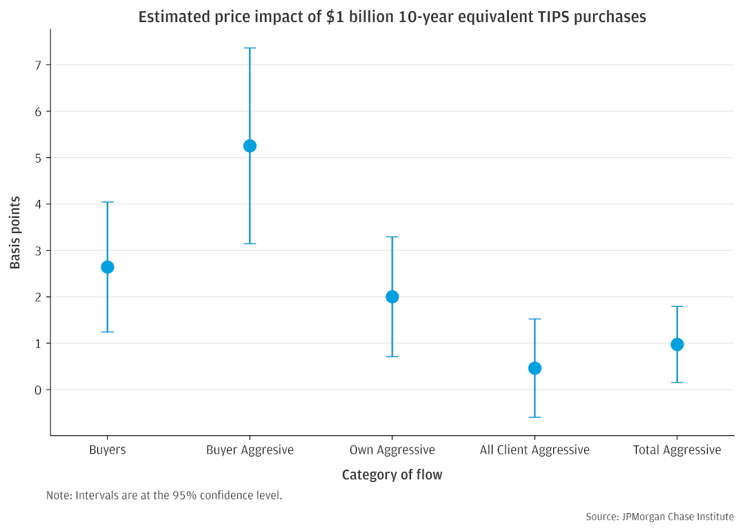
Figure B shows the estimates of aggressor flow price impact when interacting flows with the standard deviation of ten-year inflation breakeven rate changes (taken over a centered 20-day trading window and z-scored). As described in Finding 1, price impact is higher when volatility is higher. When volatility is one standard deviation below its average level, price impact is effectively zero. High volatility is associated with notably higher price impact coefficients for some aggressor flow definitions, but error bands are also wide.
Figure B: Volatility interactions show higher price impact estimates, although with wide confidence bands.
To categorize investors as chasers or contrarians in Finding 4, we run client level regressions of risk-adjusted19 flows against price action in both breakeven and real yields, as in the following regression specification. The left-hand-side variable, f, represents the risk-adjusted net flows of client, c; the 10-yr breakeven rate is BE; and the 10-year real yield is, RL.
Since market participants may respond to price changes over different tenors, we evaluate dynamics at three frequencies—daily, weekly, and monthly—across our actively trading TIPS client base from 2013 to 2019.20 To be considered active, a client would have had to conduct at least 10 TIPS trades during the sample period.
fc,t = αc +βc,BE ΔBEt +βc,RL ΔRLt + ec,t
Trend-chaser or contrarian labels are determined by the sign of significant t-statistics.21 For example, a chaser would be associated with a positive t-statistic with respect to their flows’ relationship with breakeven price action, and a negative t-statistic with respect to their relationship with real yields. We then apply our categorization to an out-of-sample period, TIPS transactions from 2020 to 2021.
The rise in prices, as measured by the price index for personal consumption expenditures, reached 5.8 percent (4.9 excluding food and energy) on a year-over-year basis as of the end of 2021, after having averaged 1.6 percent over the decade leading up to the pandemic. (Source: FRED)
See Institute Take “What do Fed rate hikes mean for U.S. households’ financial health?” (March 2022).
Our data also contains transactions for other securities traded by J.P. Morgan with its clients, including the nominal Treasury market, foreign government bonds, and foreign exchange, as explored in previous reports by the JPMorgan Chase Institute, e.g. Tracking Spillovers During the Taper Tantrum.
The infographic is a modified version of the Treasury Market Structure model appearing in Brain et al. (2018).
Financial derivatives—e.g., inflation swaps and options on inflation rates—offer traders other routes to expressing views on future inflation. However, inflation swaps in the US make up a small fraction of the volume traded in TIPS (White 2021), so we focus on transactions in the Treasury market.
See Kim, Walsh, and Wei (2019) for a concise, readable discussion of the decomposition of the yield curve across expectations and risk premia.
Our estimates derive from a dataset of de-identified institutional investor transactions in Treasury Inflation Protected Securities (TIPS) vis-à-vis J.P. Morgan. Under the assumption that these flows represent market-wide dynamics, our price impact coefficients—reported in basis points per $1 billion—should be deflated by market share, which averaged about 5 percent over the sample period.
Risks associated with making markets are higher when volatility and uncertainty are high, due to the risks of taking positions. Daley and Green (2016), for example, present a model in which asymmetric information leads to time-varying liquidity provision.
Fed transcripts from 2013 (e.g., January 2013 FOMC) cite a rule of thumb indicating that a Fed LSAP announcement of $500 billion would move the risk premium component of Treasury yields down by 15 to 20 basis points. Considering an average maturity of 5-6 years and scaling down to the TIPS market size by multiplying by one-tenth, results in an estimate of half a basis point per $1 billion ten-year equivalents. Meanwhile, Ihrig et al. (2018) and D’Amico et al. (2012) determine the impact of LSAP I to be about 1 basis point per $10 billion, a price impact the latter authors note is relatively high compared to other estimates.
For price impact of a one standard deviation flow, we multiply each aggressive flow measures’ standard deviation by its coefficient, respectively, as shown in Appendix 1, Figure A.
Kim, Walsh, and Wei (2019) provides a discussion of Fed researchers’ attempts to separate market expectations from liquidity and risk premia.
Investors with a high proportion of sales may also be liquidity demanders, but their activity would also be consistent with buying securities at auctions and selling them later in the secondary market. This would put them on-par with balanced traders.
In this analysis, we mainly weight volumes by their net duration exposure. Without trading activity, a bond portfolio loses duration over time as bonds come closer to maturity. Even passive (“buy-and-hold”) investors with no changes to their assets under management would need to be net purchasers to offset natural decline in duration.
Aggressive Buyer flows are the subset of flows of Buyers associated with “right way” movements in the relative prices of the securities traded. These can be both purchases and sales—of securities outperforming and underperforming, respectively, relative to the yield curve.
In this Finding we consider only investors with trading activity in at least 10 days in both the pre-COVID and COVID periods.
See the IAWG report documenting the events of March 2020, IAWG (2021).
See IAWG (2021) for a discussion centering on the nominal market.
Examples of institutionalized engagement with market participants include market intelligence gathering by the Federal Reserve Bank of New York’s Markets Group and the Treasury Borrowing Advisory Committee (TBAC). Studies published by the Bank for International Settlements—including Jeffery et al. (2016) and Serena et al. (2021)—provide a review of a variety of market intelligence efforts across central banks and increasing use of big data.
As discussed in the box Estimating price impact from flows data, we normalize transactions by converting the amount of interest rate risk transferred into 10-year equivalents. I.e., we consider duration-adjusted flows.
Only clients’ active trading days are included. Days with zero flow are not included.
Our cutoff is 5 percent significance level. For this exercise, we use heteroskedasticity consistent (HC2) standard errors, as suggested in Imbens and Kolesár (2016), given low regression observation counts for some market participants. In the case both coefficients are significant, we take the one with greatest statistical power.
Brain, Doug, Michiel De Pooter, Dobrislav Dobrev, Michael J. Fleming, Peter Johansson, Collin Jones, Frank M. Keane, Michael Puglia, Liza Reiderman, Anthony P. Rodrigues, and Or Shachar. 2018. “Unlocking the Treasury Market through TRACE.” Federal Reserve Bank of New York Liberty Street Economics (blog). http://libertystreeteconomics.newyorkfed.org/2018/09/unlocking-the-treasury-market-through-trace.html.
Daley, Brendan, and Brett Green. 2016. “An Information-Based Theory of Time-Varying Liquidity.” The Journal of Finance. https://doi.org/10.1111/jofi.12272.
D’Amico, S., W. English, D. López-Salido, and E. Nelson. 2012. “The Federal Reserve’s Large-scale Asset Purchase Programmes: Rationale and Effects.” Economic Journal.
Diercks, Anthony M., and Uri Carl. 2019. "A Simple Macro-Finance Measure of Risk Premia in Fed Funds Futures," FEDS Notes. Washington: Board of Governors of the Federal Reserve System. https://doi.org/10.17016/2380-7172.2305.
Gabaix, Xavier, and Ralph S. J Koijen. 2022. “In Search of the Origins of Financial Fluctuations: The Inelastic Markets Hypothesis.” SSRN Electronic Journal, n.d. https://doi.org/10.2139/ssrn.3686935.
IAWG: Interagency Working Group Report. 2021. “Recent Disruptions and Potential Reforms in the U.S. Treasury Market: A Staff Progress Report.” https://home.treasury.gov/system/files/136/IAWG-Treasury-Report.pdf.
Kim, Don, Cait Walsh, and Min Wei. 2019. "Tips from TIPS: Update and Discussions," FEDS Notes. Washington: Board of Governors of the Federal Reserve System. https://doi.org/10.17016/2380-7172.2355.
Ihrig, J., E. Klee, C. Li, M. Wei, and J. Kachovec. 2018. “Expectations about the Federal Reserve’s Balance Sheet and the Term Structure of Interest Rates.” International Journal of Central Banking.
Imbens, Guido W, and Michal Kolesár. 2016. “Robust Standard Errors in Small Samples: Some Practical Advice.” The Review of Economics and Statistics. https://doi.org/10.1162/REST_a_00552.
Jeffrey, Rosey, Holger Neuhaus, Matthew Raskin, Andreas Schrimpf, Alvin Teo, and Christian Vallence. 2016. “Market Intelligence Gathering at Central Banks.” Bank for International Settlements, Markets Committee publication. https://www.bis.org/publ/mktc08.pdf.
Serena, Jose Maria, Bruno Tissot, Sebastian Doerr, Leonardo Gambacorta. 2021. “Use of big data sources and applications at central banks.” Bank for International Settlements, Irving Fisher Committee on Central Bank Statistics (IFC). https://www.bis.org/ifc/publ/ifc_report_13.pdf.
Steel, Mark F. J. 2020. “Model Averaging and Its Use in Economics.” Journal of Economic Literature. https://doi.org/10.1257/jel.20191385.
Vayanos, Dimitri, and Jean‐Luc Vila. “A Preferred‐Habitat Model of the Term Structure of Interest Rates.” Econometrica. https://doi.org/10.3982/ECTA17440.
We thank our research team, specifically Andi Wang, Edward Biggs, and Karmen Hutchinson, for their hard work and contributions to this research. In addition, we are tremendously grateful for the many contributions of Kanav Bhagat in building the JPMorgan Chase Institute’s financial markets research group and capabilities. Additionally, we thank Emily Rapp, Stephen Harrington, Sarah Kuehl, and Preeti Vaidya for their support.
We also acknowledge the invaluable feedback we received from external experts and partners, including Jeremy Stein, Robin Greenwood, and Ralph Koijen. We are deeply grateful for their generosity of time and insights.
We are indebted to our internal partners and colleagues, who support delivery of our agenda in a myriad of ways and acknowledge their contributions to each and all releases. We would like to acknowledge Jamie Dimon, CEO of JPMorgan Chase & Co., for his vision and leadership in establishing the Institute and enabling the ongoing research agenda. We remain deeply grateful to Demetrios Marantis, Head of Corporate Responsibility, Heather Higginbottom, Head of Research & Policy, and others across the firm for the resources and support to pioneer a new approach to contribute to global economic analysis and insight.
This material is a product of JPMorgan Chase Institute and is provided to you solely for general information purposes. Unless otherwise specifically stated, any views or opinions expressed herein are solely those of the authors listed and may differ from the views and opinions expressed by J.P. Morgan Securities LLC (JPMS) Research Department or other departments or divisions of JPMorgan Chase & Co. or its affiliates. This material is not a product of the Research Department of JPMS. Information has been obtained from sources believed to be reliable, but JPMorgan Chase & Co. or its affiliates and/or subsidiaries (collectively J.P. Morgan) do not warrant its completeness or accuracy. Opinions and estimates constitute our judgment as of the date of this material and are subject to change without notice. No representation or warranty should be made with regard to any computations, graphs, tables, diagrams or commentary in this material, which is provided for illustration/reference purposes only. The data relied on for this report are based on past transactions and may not be indicative of future results. J.P. Morgan assumes no duty to update any information in this material in the event that such information changes. The opinion herein should not be construed as an individual recommendation for any particular client and is not intended as advice or recommendations of particular securities, financial instruments, or strategies for a particular client. This material does not constitute a solicitation or offer in any jurisdiction where such a solicitation is unlawful.
Wheat, Chris, George Eckerd, Shantanu Banerjee, and Melissa O’Brien. 2022. “Reading Inflation Expectations from the Treasury Market: Insights from Institutional Investor Trading Activity.” JPMorgan Chase Institute. https://www.jpmorganchase.com/insights/all-topics/financial-health-wealth-creation/treasury-market-inflation-expectations
Authors

Chris Wheat
President, JPMorganChase Institute

George Eckerd
Wealth and Markets Research Director, JPMorganChase Institute

Shantanu Banerjee
Financial Markets Research Associate

Melissa O’Brien
Data Science Lead