
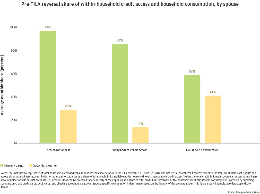
Figure 1: There were large gaps between spouses in access to credit and consumption prior to the TILA reversal.

Creating thriving communities together
See how our clients and partners—from small business owners to workforce training leaders—work with JPMorganChase to drive meaningful impact and economic growth where they live and work.
Learn moreLatest news

Veteran’s Unconventional Path to Landing her Dream Job in Tech
U.S. Army Veteran Ashley Wigfall transitioned to a civilian role and charted her path to technologist through mentorship and skills training at the JPMorgan Chase tech hub in Plano, Texas.
Learn more
Promoting equal access to consumer credit has long been a policy goal in the United States. But is credit shared equally between spouses? There are reasons to believe that disparities in credit persist within a marriage. Survey evidence shows that perceived financial inequity between spouses is among the top predictors of divorce in the U.S.1 For married couples with a single household income—roughly half of married couples with at least one child2—breadwinners likely have higher borrowing capacity than their spouses, because income determines at least part of one’s ability to borrow. However, the role of access to credit within a marriage has been understudied, and we know little about the extent and implications of credit disparities between spouses.
This research brief summarizes results published by Kim (2021), which uses de-identified JPMorgan Chase financial accounts data to document gaps between spouses in credit access and consumption.3 The research evaluates the impact of the 2013 reversal of the Truth-in-Lending-Act (TILA) on these intra-household inequalities. Before November 2013, TILA Section 150—which imposes ability-to-pay requirements in the U.S. consumer credit card market—required credit card issuers to evaluate applicants’ independent (i.e., individual) income in their lending decisions. This independent income requirement raised concerns that credit access for secondary earners or stay-at-home spouses may be restricted because these spouses had access to household income but had limited income of their own. The statute was reversed in November 2013 to allow credit card issuers to consider household income, facilitating access to credit for secondary earners and stay-at-home spouses. How did spouses differ in their access to credit and consumption patterns prior to November 2013, and did the TILA reversal changes those patterns?
Figure 1: There were large gaps between spouses in access to credit and consumption prior to the TILA reversal.
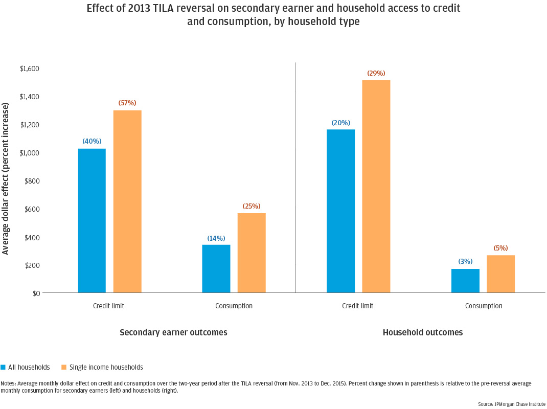
Figure 2: The 2013 TILA reversal materially increased access to credit and consumption for secondary earners and particularly within single-income households.
We use de-identified administrative data on Chase deposit account, debit card, and credit card customers to construct a sample of 66,200 opposite-sex couples from October 2012 and December 2015, covering one year before and two years after the TILA reversal. At the end of data construction steps, we have a monthly household panel dataset that tracks spending and credit card outcomes for each spouse.
To construct the sample of 66,200 households (henceforth “All Sample”), we make two types of sample restrictions: demographic and account activity. We apply the following demographic filters. We focus on individuals in working age (25 to 65 years old) as of November 2013, or when the TILA reversal was implemented. We consider two opposite-sex adults with less than 16 years of age gap and the same last name residing in the same address as a household/family unit.5 Because individuals’ marital status is not directly observed, the gender composition and age gap restrictions are applied to focus on the sample that is most likely to represent married couples. Thus, the two adults in a household unit are assumed to be a married couple. Note that this sample restriction leaves many other types of household units, such as domestic partnership, same-sex couples, cohabiting couples, married couples with different last names, or married couples that live apart, among others.
Using this sample of two adult-member households, we apply the following account activity filters. We focus on spouses who are either a primary or secondary account holder of at least one active (i.e., having at least 5 transactions every month) Chase personal checking account. Since we do not require each spouse to have a separate checking account, this sample captures a wide range of account structure types, such as couples with only one joint checking account as well as those with both joint and separate accounts. For couples with joint accounts, we require spouses to have their own debit card associated with these shared accounts to be able to track each spouse’s spending on the joint accounts. We further restrict the sample to couples that make above poverty threshold annual labor income in 2013.6 We require at least one spouse to have a Chase personal credit card. Finally, we focus on couples where secondary earners did not have a sole Chase personal credit card account as of the beginning of the sample period (October 2012). This restriction allows us to focus on a sample of new credit card openers who are required to report income on their credit card applications around the TILA reversal.
We create a subsample of roughly 11,700 households (henceforth “Card Holder Sample”) where secondary earners eventually opened a sole personal Chase credit card at some point during the sample period. This helps to focus on the subsample of households where the credit gap between spouses eventually changed following the TILA reversal. For detailed rationale behind sample construction criteria and variable construction method, see Kim (2021) Section 4.
See Dew, Britt, and Huston (2012) for survey evidence.
Source: U.S. Bureau of Labor Statistics. This statistic refers to the share of non-dual income households amongst consumer units that reported having a spouse and at least one child under age 18.
This study considers two opposite-sex adults with less than 16 years of age gap and the same last name and address as a household/family unit. The two adults in a household unit are assumed to be a married couple. This sample restriction leaves many other types of household units, such as same-sex couples, cohabiting couples, married couples with different last names, or married couples that live apart.
See the measurement section in data appendix for how stay-at-home spouses are defined.
Note that researchers do not directly observe individuals’ address and family names as they are de-identified.
$17,000 is the U.S. Department of Health and Services’ 2013 poverty threshold for two-member household.
For example, if a joint checking account shows an electronic bill payment of $100, we attribute $50 to one spouse and $50 to the other spouse.
Given that wage earners typically receive income on a bi-weekly basis (U.S. Bureau of Labor Statistics, 2020), the frequency of payroll deposits and the payroll difference between spouses helps to identify double income households.
We thank our research team for their hard work and contribution to this research, in particular, Damon Swaner in Consumer Banking & Fraud for sharing his insights on the TILA reversal and how it was implemented in practice. Additionally, we thank Emily Rapp, Annabel Jouard and Kristine Pham for their support. We are indebted to our internal partners and colleagues, who support delivery of our agenda in a myriad of ways, and acknowledge their contributions to each and all releases.
We are also grateful for the invaluable constructive feedback we received from external experts and partners. We are deeply grateful for their generosity of time, insight, and support.
We would like to acknowledge Jamie Dimon, CEO of JPMorgan Chase & Co., for his vision and leadership in establishing the Institute and enabling the ongoing research agenda. We remain deeply grateful to Peter Scher, Vice Chairman, Demetrios Marantis, Head of Corporate Responsibility, Heather Higginbottom, Head of Research & Policy, and others across the firm for the resources and support to pioneer a new approach to contribute to global economic analysis and insight.
This material is a product of JPMorgan Chase Institute and is provided to you solely for general information purposes. Unless otherwise specifically stated, any views or opinions expressed herein are solely those of the authors listed and may differ from the views and opinions expressed by J.P. Morgan Securities LLC (JPMS) Research Department or other departments or divisions of JPMorgan Chase & Co. or its affiliates. This material is not a product of the Research Department of JPMS. Information has been obtained from sources believed to be reliable, but JPMorgan Chase & Co. or its affiliates and/or subsidiaries (collectively J.P. Morgan) do not warrant its completeness or accuracy. Opinions and estimates constitute our judgment as of the date of this material and are subject to change without notice. No representation or warranty should be made with regard to any computations, graphs, tables, diagrams or commentary in this material, which is provided for illustration/reference purposes only. The data relied on for this report are based on past transactions and may not be indicative of future results. J.P. Morgan assumes no duty to update any information in this material in the event that such information changes. The opinion herein should not be construed as an individual recommendation for any particular client and is not intended as advice or recommendations of particular securities, financial instruments, or strategies for a particular client. This material does not constitute a solicitation or offer in any jurisdiction where such a solicitation is unlawful.
Greig, Fiona, Olivia Kim. 2022. “Credit and the Family: The Economic Consequences of Closing the Credit Gap of US Couples” JPMorgan Chase Institute. https://www.jpmorganchase.com/insights/all-topics/financial-health-wealth-creation/credit-and-the-family-truth-in-lending-act
Authors

Fiona Greig
Former Co-President

Olivia Kim