Findings

01

Payment reduction for borrowers with similar payment burdens varied by two to three times across different modification programs.

Borrowers with similar payment burdens (as measured by pre-modification mortgage payment-to-income ratio, or PTI) received considerably different payment reductions depending on the modification they received:

  • Borrowers with a high mortgage PTI (above 50 percent) received more than twice the payment reduction from HAMP (55 percent) compared to the GSE program (27 percent).*
  • Borrowers with a low mortgage PTI received three times the payment reduction from the GSE program (25 percent) compared to HAMP (8 percent).

*HAMP refers to the Home Affordable Modification Program introduced by the Federal Government and the GSE program refers to the proprietary modifications offered by the Government Sponsored Enterprises Fannie Mae and Freddie Mac.

Bar graph shows pre-modification mortgage payment-to-income ratio.

FINDING ONE

Payment reduction for borrowers with similar payment burdens varied by two to three times across different modification programs.

Borrowers with a high mortgage payment-to-income ratio are classified as those who spend 50 to 70 percent of their income on mortgage payments. For these borrowers, GSE programs reduced payments by 27 percent, while HAMP reduced payments by 55 percent.

Borrowers with a low mortgage payment-to-income ratio are classified as those who spend 30 to 33 percent of their income on mortgage payments. For these borrowers, GSE programs reduced payments by 25 percent, while HAMP reduced payments by 8 percent.

Source: JPMorgan Chase Institute

01

A 10 percent mortgage payment reduction reduced default rates by 22 percent.

Infographic showing that a 10 percent mortgage payment reduction reduced default rates by 22 percent.

FINDING TWO

A 10 percent mortgage payment reduction reduced default rates by 22 percent.

Source: JPMorgan Chase Institute

01

For borrowers who remained underwater, mortgage principal reduction had no effect on default.

There was no difference between the post-modification default rates of borrowers who received principal plus payment reduction and borrowers who received only payment reduction. This finding suggests that “strategic default” was not the primary driver of default decisions for these underwater borrowers, meaning that they were not defaulting simply because they owed more on their mortgage than their house was worth.

Line graph shows cumulative default rate.

FINDING THREE

For borrowers who remained underwater, mortgage principal reduction had no effect on default.

There was no difference between the post-modification default rates of borrowers who received principal plus payment reduction and borrowers who received only payment reduction. This finding suggests that “strategic default” was not the primary driver of default decisions for these underwater borrowers, meaning that they were not defaulting simply because they owed more on their mortgage than their house was worth.

The below data utilizes a 95% confidence interval. Because the two confidence intervals overlap, the two cumulative default rates are not statistically different from each other.

Cumulative Default Rate: Payment Reduction

Months since modification Coefficient 95% Confidence Interval Low 95% Confidence Interval High
0 0.2% -0.5% 1.5%
1 0.3% -0.5% 1.5%
2 0.4% -0.4% 1.5%
3 0.8% 0.1% 1.5%
4 1.0% 0.3% 1.5%
5 1.2% 0.5% 1.5%
6 1.5% 0.8% 1.5%
7 1.7% 1.0% 1.5%
8 2.1% 1.4% 1.5%
9 2.5% 1.7% 1.5%
10 2.9% 2.1% 1.5%
11 3.1% 2.4% 1.5%
12 3.5% 2.8% 1.5%
13 4.0% 3.2% 1.5%
14 4.4% 3.7% 1.5%
15 4.9% 4.2% 1.5%
16 5.3% 4.6% 1.5%
17 5.7% 4.9% 1.5%
18 6.2% 5.5% 1.5%
19 6.8% 6.0% 1.5%
20 7.2% 6.4% 1.5%
21 7.5% 6.8% 1.5%
22 7.9% 7.2% 1.5%
23 8.3% 7.6% 1.5%
24 8.7% 8.0% 1.5%

Cumulative Default Rate: Payment + Principal Reduction

Months since modification Coefficient 95% Confidence Interval Low 95% Confidence Interval High
0 0.0% -1.2% 2.6%
1 0.0% -1.2% 2.6%
2 0.1% -1.1% 2.6%
3 0.3% -0.9% 2.6%
4 0.6% -0.7% 2.6%
5 0.9% -0.4% 2.6%
6 1.1% -0.1% 2.6%
7 1.5% 0.2% 2.6%
8 1.6% 0.3% 2.6%
9 1.9% 0.6% 2.6%
10 2.4% 1.1% 2.6%
11 3.0% 1.7% 2.6%
12 3.5% 2.2% 2.6%
13 3.9% 2.7% 2.6%
14 4.3% 3.0% 2.6%
15 4.8% 3.5% 2.6%
16 5.0% 3.7% 2.6%
17 5.6% 4.3% 2.6%
18 5.8% 4.5% 2.6%
19 6.1% 4.8% 2.6%
20 6.3% 5.1% 2.6%
21 6.6% 5.4% 2.6%
22 7.0% 5.7% 2.6%
23 7.2% 5.9% 2.6%
24 7.3% 6.1% 2.6%

Source: JPMorgan Chase Institute

01

For borrowers who remained underwater, mortgage principal reduction had no effect on consumption.

There was no difference in the post-modification credit card spending of borrowers who received principal plus payment reduction and borrowers who received only payment reduction relative to their spending 12 months before modification.

Line graph shows average credit card spending around modification

FINDING FOUR

For borrowers who remained underwater, mortgage principal reduction had no effect on consumption.

There was no difference in the post-modification credit card spending of borrowers who received principal plus payment reduction and borrowers who received only payment reduction relative to their spending 12 months before modification.

Months since modification Payment + Principal Reduction Payment Reduction
-12 $222 $265
-11 $209 $254
-10 $202 $242
-9 $200 $250
-8 $198 $247
-7 $208 $237
-6 $208 $222
-5 $193 $227
-4 $188 $234
-3 $184 $221
-2 $192 $229
-1 $189 $228
0 $194 $227
1 $189 $224
2 $197 $230
3 $199 $220
4 $190 $239
5 $215 $244
6 $198 $242
7 $201 $243
8 $212 $248
9 $204 $241
10 $210 $250
11 $201 $243
12 $208 $244

Source: JPMorgan Chase Institute

01

Default was correlated with income loss, regardless of debt-to-income ratio or home equity.

Mortgage default closely followed a substantial drop in income. This pattern held regardless of pre-modification mortgage PTI or loan-to-value (LTV) ratio, suggesting that it was an income shock rather than a high payment burden or negative home equity that triggered default.

Line graph shows a change in monthly income and mortgage payment made from baseline

FINDING FIVE

Default was correlated with income loss, regardless of debt-to-income ratio or home equity.

Mortgage default closely followed a substantial drop in income. This pattern held regardless of pre-modification mortgage PTI or loan-to-value (LTV) ratio, suggesting that it was an income shock rather than a high payment burden or negative home equity that triggered default.

Months since default Income Mortgage payment
-12 0 0
-11 78 13
-10 39 19
-9 28 19
-8 103 29
-7 56 16
-6 -14 6
-5 -82 -9
-4 -212 -35
-3 -355 -103
-2 -520 -330
-1 -649 -391
0 -620 -712
1 -210 -135
2 -234 -236
3 -233 -224
4 -196 -219
5 -244 -223
6 -241 -209
7 -263 -199
8 -282 -199
9 -258 -191
10 -275 -202
11 -279 -206
12 -262 -197

Source: JPMorgan Chase Institute

Data

From a universe of over 1 million Chase mortgage customers who received a modification, we created a data asset of 450,000 de-identified modification recipients.

Infographic describing the data asset used for the research.

DATA

From a universe of over 1 million Chase mortgage customers who received a modification, we created a data asset of 450,000 de-identified mortgage customers who met the following three sampling criteria:

1. Received a modification from one of the following:

  • The Home Affordable Modification Program introduced by the Federal Government
  • A modification program of the Government Sponsored Enterprises Fannie Mae and Freddie Mac
  • A Chase proprietary modification program

2. Modification completed between July 2009 and June 2015

3. First modifications only

We limit our sample to first modifications only because we would expect subsequent modifications to be different along many observable and unobservable dimensions.

A subset of these Chase customers also had a Chase credit card and/or a Chase checking account, which provided a unique lens on the relationships between mortgage modifications, default, credit card spending, and income.

Source: JPMorgan Chase Institute

Conclusion

In this report, we measured the impact of mortgage payment and principal reduction on default and consumption. Our results have implications for both housing policy and monetary policy.

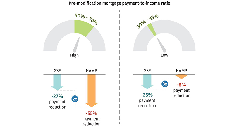
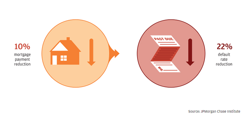
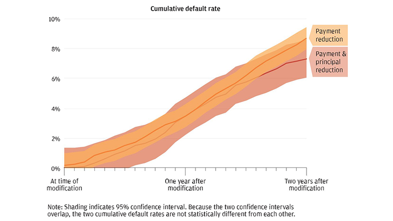
Our findings suggest that mortgage modification programs that are designed to target substantial payment reduction will be most effective at reducing mortgage default rates. Modification programs designed to reach affordability targets based on debt-to-income measures without regard to payment reduction will be less effective. Principal focused mortgage debt reduction programs that target a specific LTV ratio but leave borrowers underwater will also be less effective at reducing defaults.

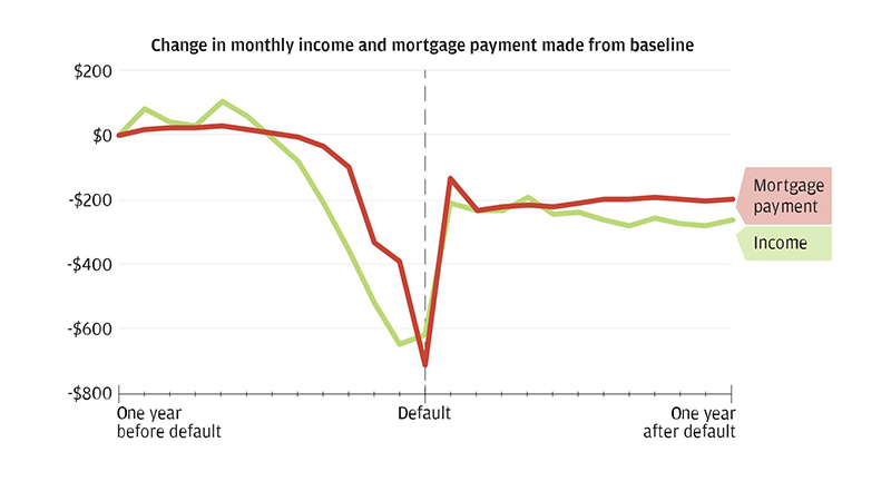
To the extent that a mortgage modification can be considered a re-origination, our findings may have application to underwriting standards as well. The fact that default was correlated with income loss provides evidence that static affordability measures such as debt-to-income ratio were not a good predictor of default. Both high and low mortgage PTI borrowers experienced a similar income drop just prior to default, suggesting that even among those borrowers whose mortgages would be categorized as unaffordable by conventional standards, it was a drop in income rather than a high level of payment burden that triggered default. Therefore, policies that help borrowers establish and maintain a suitable cash buffer that can be drawn down in the event of an income shock or an expense spike could be an effective tool to prevent mortgage default.

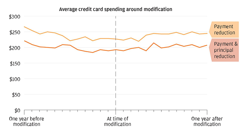
The housing wealth effect is one of the important mechanisms that transmits changes in monetary policy to household consumption. This transmission mechanism relies on accommodative monetary policy leading to higher house prices, and the increase in housing wealth that in turn stimulates consumption. The lack of consumption response from underwater borrowers to principal reductions suggests that the marginal propensity to consume out of housing wealth is nearly zero for these homeowners. For underwater borrowers, the inability to translate increased home equity into liquid resources (e.g., through equity extraction) may nullify the housing wealth effect and thus constrain this transmission mechanism.

Authors

Diana Farrell

Diana Farrell

Founding and Former President & CEO

Kanav Bhagat

Kanav Bhagat

Director of Financial Markets Research | JPMorgan Chase Institute

Pascal Noel

Pascal Noel

Neubauer Family Assistant Professor of Finance at the University of Chicago Booth School of Business

Peter Ganong

Peter Ganong

Assistant Professor at the University of Chicago Harris School of Public Policy